Click to show original
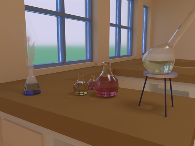
This is my final project for CSE 168! Ultimately, I implemented rough dielectrics and volumetric fog—including both absorption/attenuation and scattering.
These effects can be seen in the hero image above. The bottles are all regular dielectrics, and the window panes are slightly roughened glass. Inside of the bottles, you can see liquid that has different levels of attenuation for different colors, creating colored caustics on the bench. Finally, the blue and greenish-yellow bottles have homogenous fog in them, with the blue bottle having it escape into the air.
Before attempting to implement more physical dielectrics, I knew it would be helpful to create perfect ones.
To this end, I created the DielectricPerfect.cpp. Because this is a delta function, I also added
a field to the material struct that lets the renderer know not to try to use a PDF function to alter
the throughput.
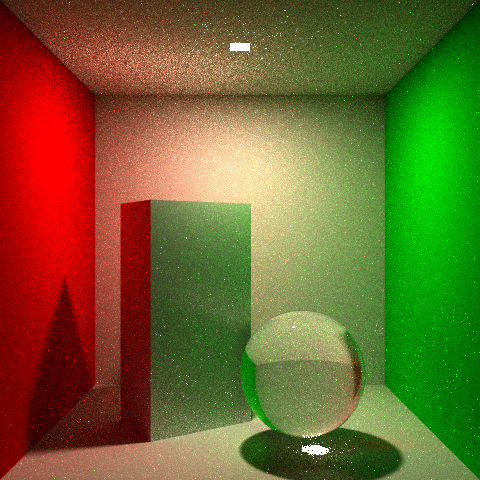
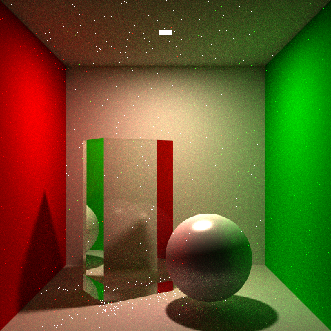
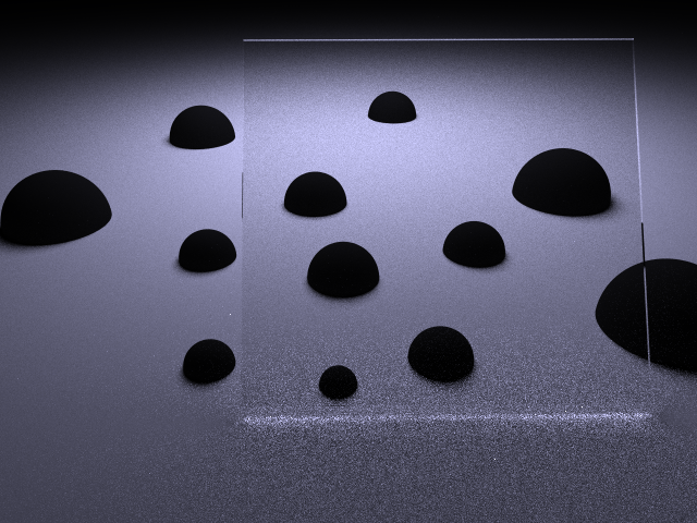
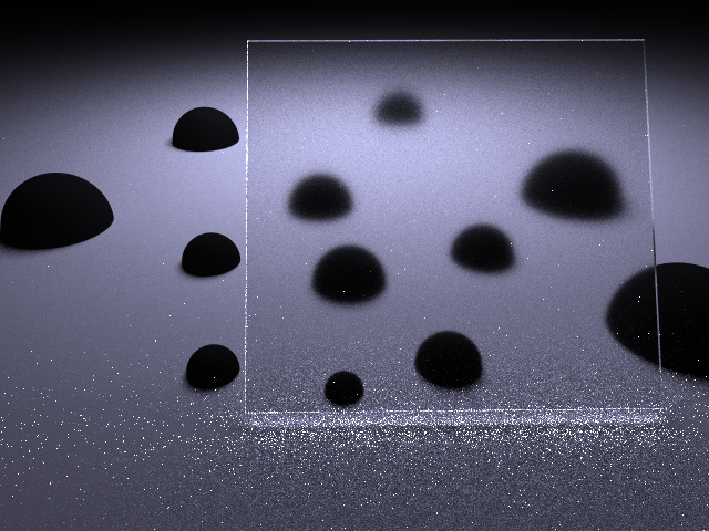
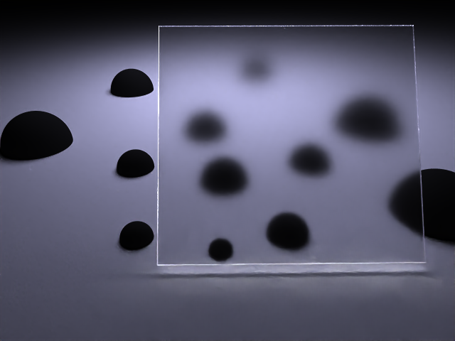
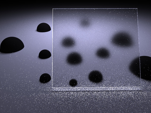
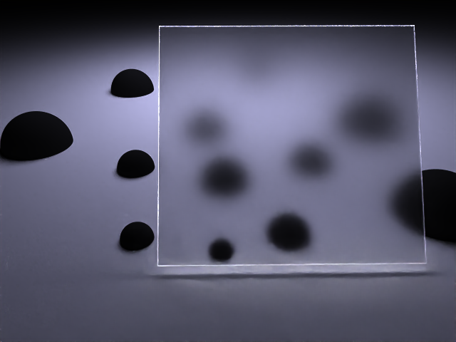
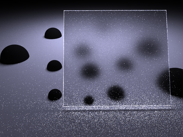
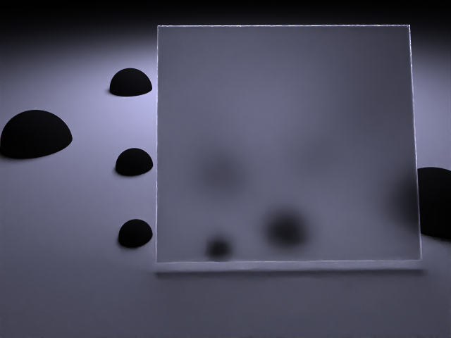
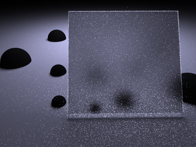
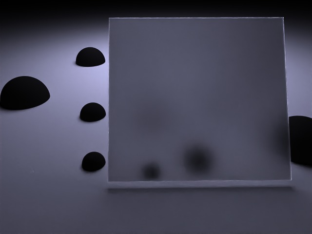
Below are some examples I rendered with this material. These images were rendered at 256 spp and then denoised with OIDN. Because the OIDN images look so much cleaner, they are the ones I show immediately, though I have also included the original images in a dropdown below.
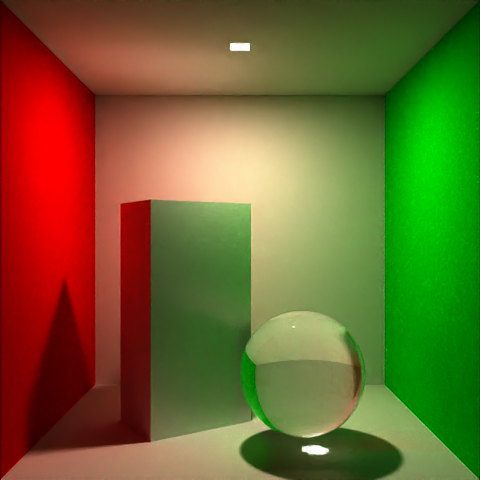
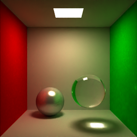
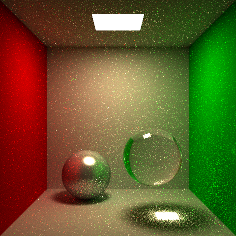
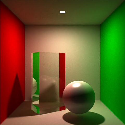
The ultimate goal of doing the above section was really to create more realistic dielectrics that have a rough surface by combining transmission with the GGX model. This paper gives a good overview of how to extend the GGX model to dielectrics.
It is also from this paper I got the inspiration for how to display the different roughness levels. I used the values they had in their Figure 15 (anti-glare, ground, and etched), plus came up with some values in between to show the transition from smooth to rough better.
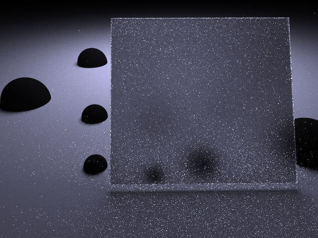
Standard Perfect Dielectric (α=0.000)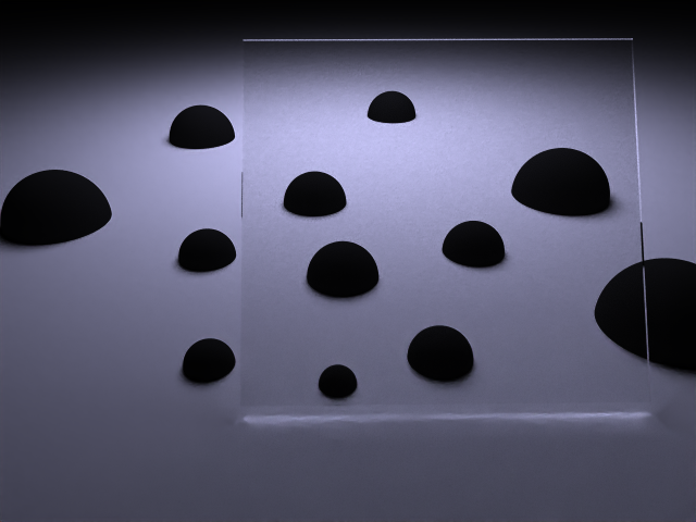
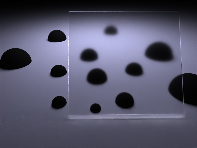
In addition to the class slides on the topic, I used this source to get some more information about how volumetrics work.
My first step was to implement volume absorption. I do this by specifying the
value of σ_a (the absorption coefficient) on the backface of different
triangles, which then becomes part of the material similarly to diffuse and specular colors.
I then keep track of the medium the current material is traveling through by adding and subtracting
these values as it enters and exits materials. To this end, I also added a Volume BRDF that
effectively just keeps the ray going forward but lets me adjust the value of the current absorption coefficient.
Using this coefficient, we can have an exponential falloff of the throughput as the ray travels through the medium.
The initial results were very noisy! This is because our previous version of NEE doesn't account for materials that are passable, effectively removing it when behind a volume. Note that this is also a problem for dielectrics, but for volumes we can actually mostly handle it because the rays don't bend as they travel through the medium (scattering is a slight problem, and I'm not fully sure how to handle this case).
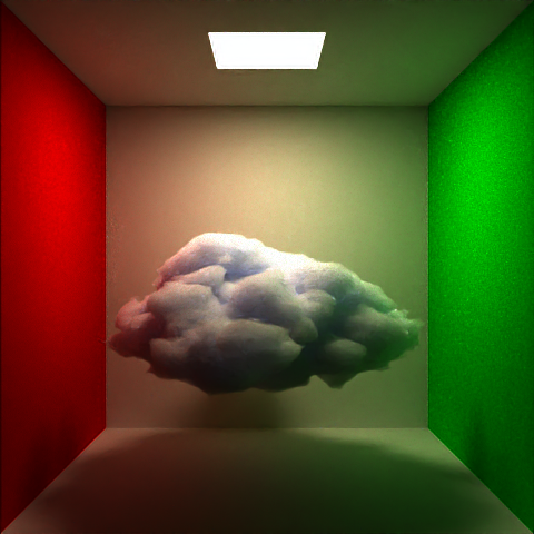
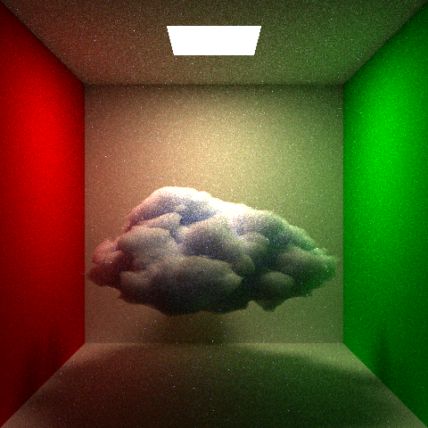
Results before and after updating NEE, spp=64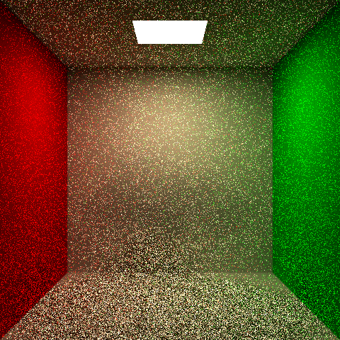
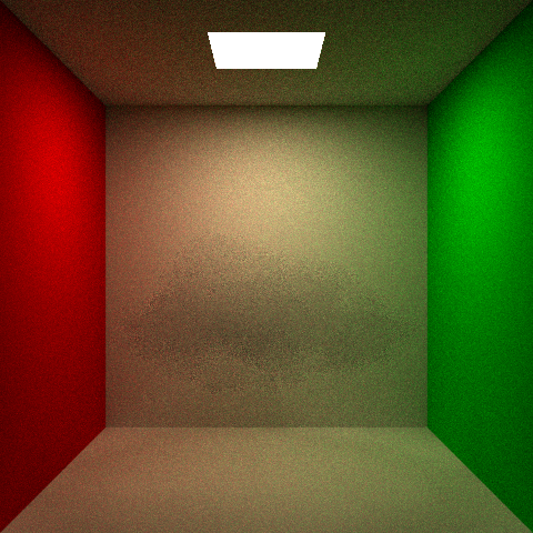
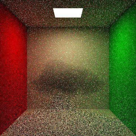
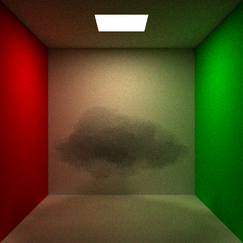
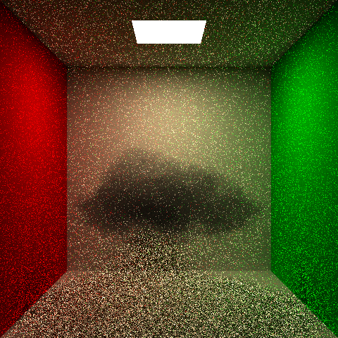
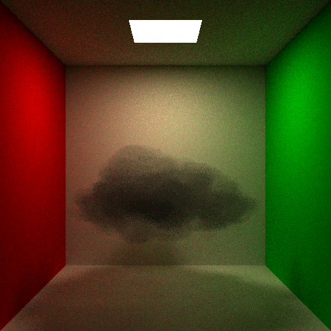
Now that NEE works properly, we can generate images with the cloud at different values of σ_a.
Note that we're doing this at only 64 spp because absorption doesn't introduce very much noise.
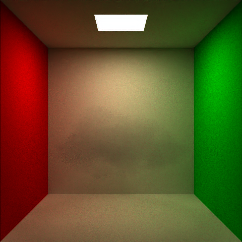
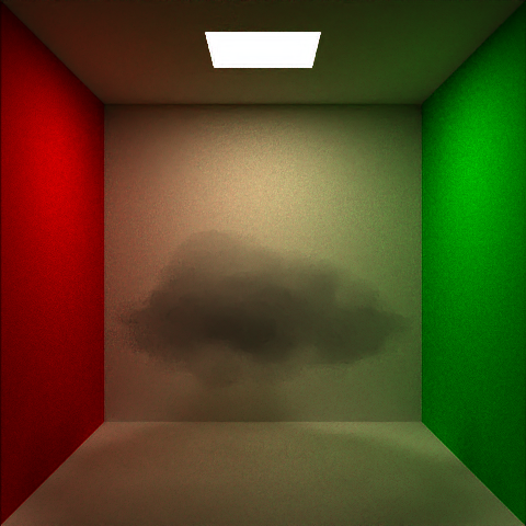
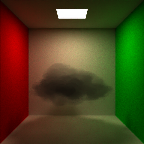
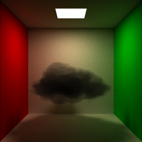
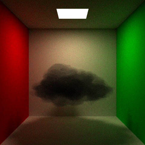
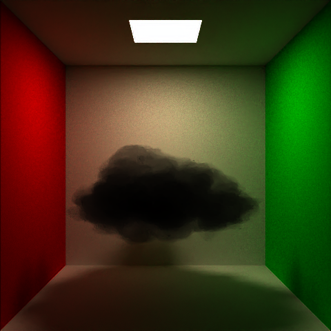
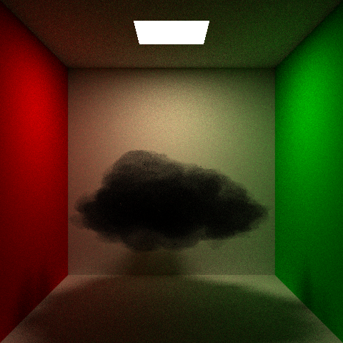
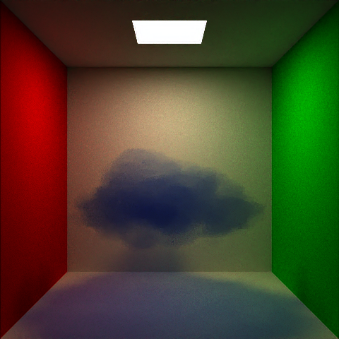
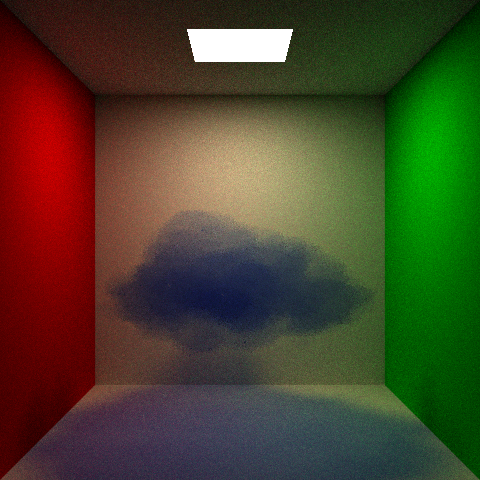
We can also use different values of σ_a for the different colors, allowing us
to create things like colored smoke and stained glass.
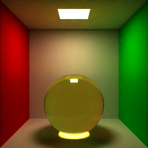
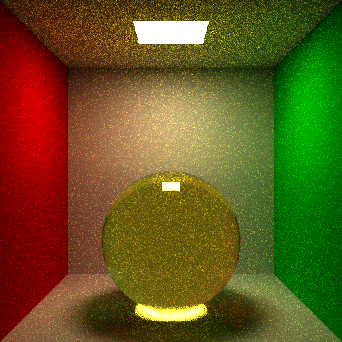
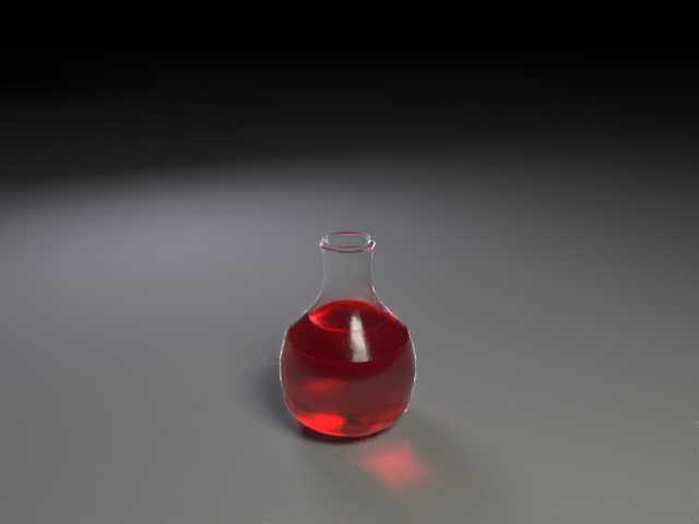
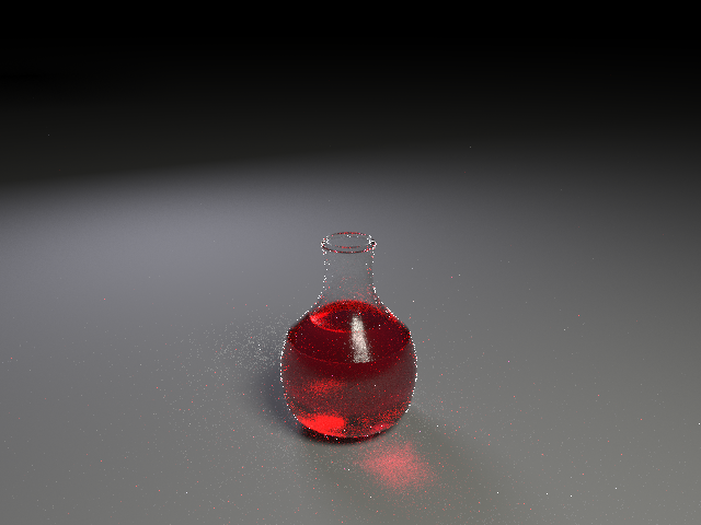
Finally, I needed to implementing volumetric scattering, which is the primary effect at play in clouds and white fog.
Typical implementations will combine σ_s (the scattering coefficient) and
σ_a into a single coefficient σ_t, which is then used to
determine when the next scattering/absorption event happens. However, in my case I actually separated
them because I only trace a single ray for all colors and combining them would make it harder to account
for attenuation for different colors.
To this end, I calculate when the next scattering event would happen by sampling an exponential distribution
with σ_s and see if that's closer than the next object hit. I then always apply the exponential
absorption effect on throughput, no matter whether we had a scattering hit or not.
For the scattering event, I sample from the Henyey-Greenstein function to determine where the ray scatters to,
using g=0.85 (a reasonable value for clouds).
Something to note is that for these example images, the value of σ_s is higher than what we'd expect.
However, I think this is because the size of the cloud is much much smaller than the real size of a cloud, so we
need to force the scattering events to happen more frequently to get the same effect we expect. There is a bit more randomness
at play here, so I used 128 spp.
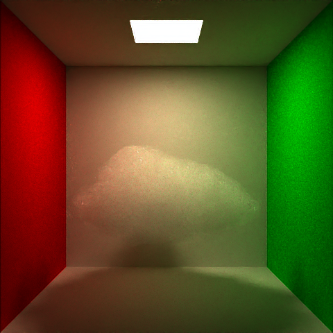
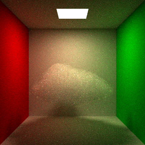
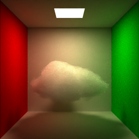
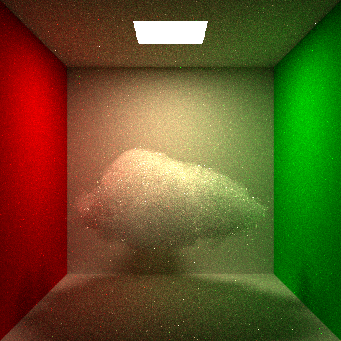
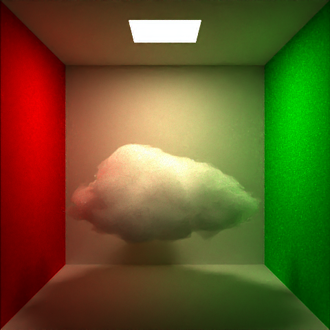
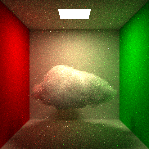
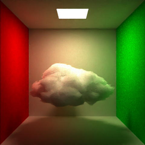
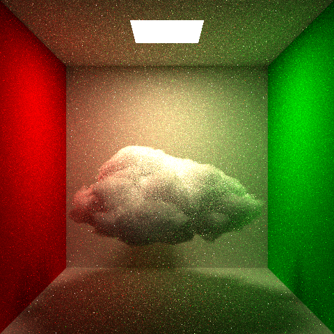
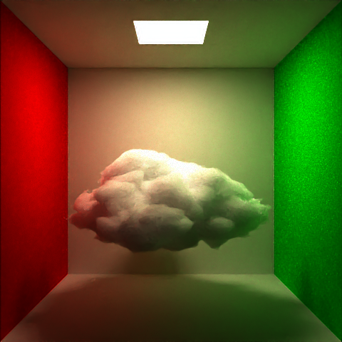
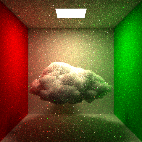
We can also of course combine the effects of absorption and scattering, which can give us something like this blue cloud for our final image.
Blue Cloud